Preterm infants’ pose estimation with spatio-temporal features
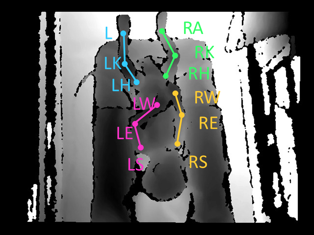
Objective. Preterm infants’ limb monitoring in neonatal intensive care units (NICUs) is of primary importance for assessing infants’ health status and motor/cognitive development. Herein, we propose a new approach to preterm infants’ limb pose estimation that features spatio-temporal information to detect and track limb joints from depth videos with high reliability. Methods. respectively.
Sara Moccia, Lucia Migliorelli, Virgilio Carnielli, and Emanuele Frontoni, Member, IEEE
Abstract — Limb-pose estimation is performed using a deeplearning framework consisting of a detection and a regression convolutional neural network (CNN) for rough and precise joint localization. The CNNs are implemented to encode connectivity in the temporal direction through 3D convolution. Assessment of the proposed framework is performed through a comprehensive study with sixteen depth videos acquired in the actual clinical practice from sixteen preterm infants (the babyPose dataset). Results. When applied to pose estimation, the median root mean square distance, computed among all limbs, between the estimated and the ground-truth pose was 9.06 pixels, overcoming approaches based on spatial features only (11.27 pixels). Conclusion. Results showed that the spatio-temporal features had a significant influence on the pose-estimation performance, especially in challenging cases (e.g., homogeneous image intensity). Significance. This paper significantly enhances the state of art in automatic assessment of preterm infants’ health status by introducing the use of spatio-temporal features for limb detection and tracking, and by being the first study to use depth videos acquired in the actual clinical practice for limb-pose estimation. The babyPose dataset has been released as the first annotated dataset for infants’ pose estimation.
Index Terms — Preterm infants, spatio-temporal features, deep learning, pose estimation, convolutional neural networks.
I. INTRODUCTION
RETERM birth is defined by the World Health Organization as a birth before thirty-seven completed weeks of gestation. In almost all high-income Countries, complications of preterm birth are the largest direct cause of neonatal deaths, accounting for the 35% of the world deaths a year [1]. The effects of preterm birth among survivor infants may have impact throughout life. In fact, preterm birth may compromise infants’ normal neuro-developmental functioning, e.g., by increasing the risk of cerebral palsy.
Clinicians in neonatal intensive care units (NICUs) pay particular attention to the monitoring of infants’ limbs, as to have possible hints for early diagnosing cerebral palsy [2]. However, this monitoring still relies on qualitative and sporadic observation of infants’ limbs directly at the crib (e.g., using qualitative scales [3], [4]). Beside being time-consuming, it may be prone to inaccuracies due to clinicians’ fatigue and susceptible to intra- and inter-clinician variability [5]. This further results in a lack of documented quantitative parameters on the topic, while in closer fields, such as metabolic and respiratory monitoring, a solid clinical literature already exists [6], [7].
This work was supported by the European Union through the grant SINC – System Improvement for Neonatal Care under the EU POR FESR 14-20 funding program. (Corresponding author: Sara Moccia).S. Moccia is with the Department of Information Engineering, Universita Politecnica delle Marche, Ancona (Italy) and with the Department of` Advanced Robotics, Istituto Italiano di Tecnologia, Genoa (Italy) e-mail: s.moccia@univpm.itL. Migliorelli and E. Frontoni are with the Department of InformationEngineering, Universita Politecnica delle Marche, Ancona (Italy)`V. Carnielli is with the Department of Neonatology, University Hospital Ancona, Universita Politecnica delle Marche, Ancona, Italy`
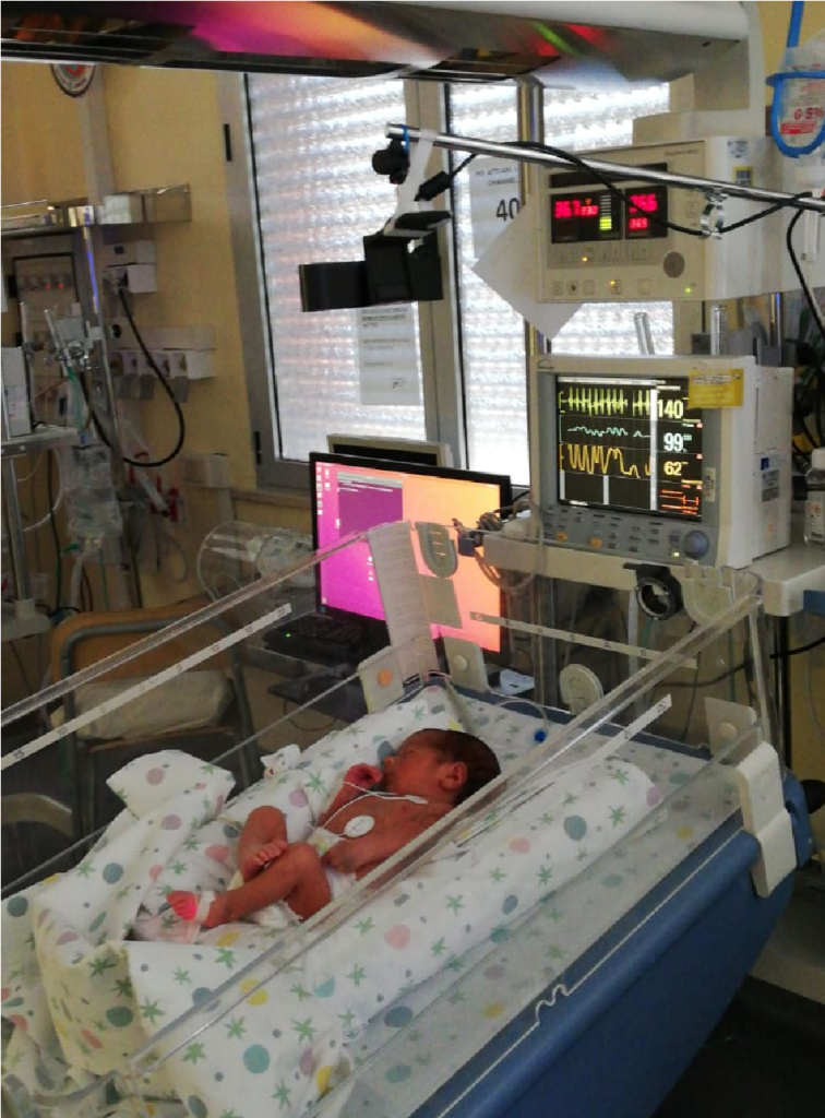
A possible solution to attenuate the problem of qualitative monitoring could be to develop an automatic video-based system for infants’ limb-pose estimation and tracking. This would support clinicians in the limb monitoring process without hindering the actual clinical practices: the camera could be positioned on top of infants’ crib (Fig. 1) leaving health operators free to move and interact with the infants. Estimating limb pose, however, is not a trivial task, considering that there may be small and barely visible joints, as well as presence of occlusions, lighting changes and infants’ movements. To tackle these issues, researches in the closer fields relevant to video analysis (e.g., [8], [9], [10]) have recently pointed out the benefits of including temporal information in their analysis. Thus, guided by the research hypothesis that spatio-temporal features extracted from depth videos may boost performance with respect to spatial features alone, the contributions of this paper are summarized as follows:
1) Estimation of infants’ limb pose from depth videos
(Sec. II): Development of an innovative deep learning framework for preterm infants’ pose estimation, which exploits spatio-temporal features for automatic limb-joint detection and connection;
2) Validation in the actual clinical practice (Sec. III): A
comprehensive study is conducted using 16 videos (16000 frames) acquired in the actual clinical practice from 16 preterm infants (the babyPose dataset) to experimentally investigate the research hypothesis.
To the best of our knowledge, this is the first attempt to investigate spatio-temporal features for automatic infants’ pose estimation from videos acquired in the actual clinical practice. It is worth noting that we intentionally focused our analysis on depth videos (instead of RGB ones) to address concerns relevant to infant privacy protection [11]. We made our babyPose dataset and code fully available online1.
A. Related work
In the past decades, a number of computer-based approaches was developed to support clinicians in monitoring infants’ limb. In [12] and [13], wearable sensors placed on wrists and knees are used, respectively. Data from tri-axial accelerometer, gyroscope, and magnetometer (integrated in the sensor) are processed to monitor infants’ limb movement via a thresholdsensitive filtering approach, achieving encouraging results. However, practical issues may arise when using wearable sensors. Hence, even though miniaturized, these sensors are directly in contact with the infants, possibly causing discomfort, pain and skin damage while hindering infant’s spontaneous movements [14].

To attenuate these issues, great efforts have been spent on unobstructive monitoring solutions (e.g., video data from RGB or RGB-D cameras). Preliminary results are achieved in [15] and [16] for infant’s whole-body segmentation with threshold-based algorithms. However, as highlighted in [17], monitoring each limb individually is crucial to assist clinicians TABLE I: Table of symbols used in Sec. II.
| Symbol | Description |
| Ω | Frame domain |
| C | Number of connections |
| H | Frame height |
| J | Number of joints |
| LCE | Binary cross-entropy loss |
| LMSE | Mean squared error loss |
| rd | Radius for detection joint-map generation |
| W | Frame width |
| Wd | Number of frames along the temporal direction |
| Ws | Frame overlap along the temporal direction |
in the health-assessment process. With such a view, in [18] RGB images are processed to detect infant’s limb skeleton with a learning-based approach. The histogram of oriented gradients is used as feature to train a structured support vector machine aimed at retrieving limb joints, which are then connected knowing the spatial relations between infants’ body parts. Following the learning paradigm, and inspired by recent consideration that showed the potentiality of deep learning over standard machine learning [19], in a preliminary work [20], we investigated the use of a convolutional neural network (CNN) for roughly detecting limb joints and joint connections, followed by a 2D regression CNN for accurate joint and joint-connection position estimation.
All these approaches only consider spatial features, without exploiting the temporal information that, however, is naturally encoded in video recordings [10]. A first attempt of including temporal information is proposed in [21], where RGB videos are processed by a semi-automatic algorithm for single-limb tracking. Motion-segmentation strategies based on particle filtering are implemented, which, however, relies on prior knowledge of limb trajectories. Such trajectories may have high variability among infants, especially in case of pathology, hampering the translation of the approach into the actual clinical practice. A possible alternative to exploit temporal information could be using 3D CNNs to directly extract spatiotemporal information from videos, which has already been shown to be robust in action recognition [22] as well as for surgical-tool detection [8]. Following this consideration, in this work we propose a framework based on 3D CNNs for estimating preterm infants’ limb pose from depth video recordings acquired in the actual clinical practice.
II. METHODS
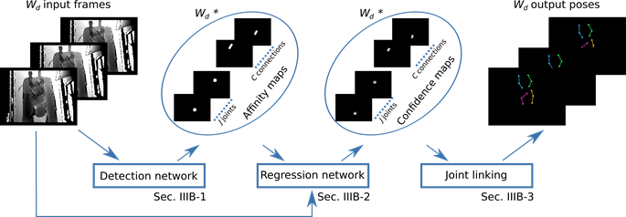
Figure 2 shows an overview of the workflow of the proposed spatio-temporal framework for preterm infants’ pose estimation from depth videos (Sec. II-B). We exploit two consecutive CNNs, the former for detecting joints and joint connections, resulting in what we call affinity maps (Sec. II-B1), and the latter for precisely regressing the joint position, resulting in the so-called confidence maps, by exploiting both the joint and joint-connection affinity maps, with the latter acting as guidance for joint linking (Sec. II-B2).
The joints belonging to the same limb are then connected using bipartite graph matching (Sec. II-B3). The pose-estimation framework relies on modeling limb joints as depicted in Fig. 3 and explained in Sec. II-A. Table I lists the symbols used in Sec. II.
A. Infants’ joint model and data preparation
The proposed infant’s model considers each of the 4 limbs as a set of 3 connected joints (i.e., wrist, elbow and shoulder for arms, and ankle, knee and hip for legs), as shown in Fig. 3. This choice is driven by clinical considerations: as introduced in Sec. I, monitoring legs and arms is of particular interest for evaluating preterm infants’ cognitive and motor development [23], [24].
With the aim of extracting spatio-temporal features, instead of considering depth frames individually as in [20], we adopt temporal clips. Following the approach presented in [8], we use a sliding window algorithm for building the clips: starting from the first video frame, an initial clip with a predefined number (Wd) of frames is selected and combined to generate a 4D datum of dimensions frame width (W) x frame height (H) x Wd x 1, where 1 refers to the depth channel. Then the window moves of Ws frames along the temporal direction and a new clip is selected.
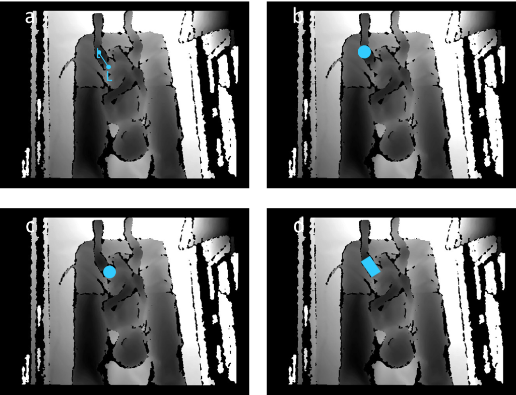
To train the detection CNN, we perform multiple binarydetection operations (considering each joint and jointconnection separately) to solve possible ambiguities of multiple joints and joint connections that may cover the same frame portion (e.g., in case of self-occlusion). Hence, for each depth-video frame, we generate 20 binary ground-truth affinity maps: 12 for joints and 8 for joint connections (instead of generating a single mask with 20 different annotations, which has been shown to perform less reliably [25]). Sample groundtruth maps are shown in Fig. 4. This results in a 4D datum of size W x H x Wd x 20. For each affinity map, we consider a region of interest consisting of all pixels that lie in the circle of a given radius (rd) centered at the joint center. A similar approach is used to generate the ground-truth affinity map for the joint connections. In this case, the ground-truth is the rectangular region with thickness rd and centrally aligned with the joint-connection line.
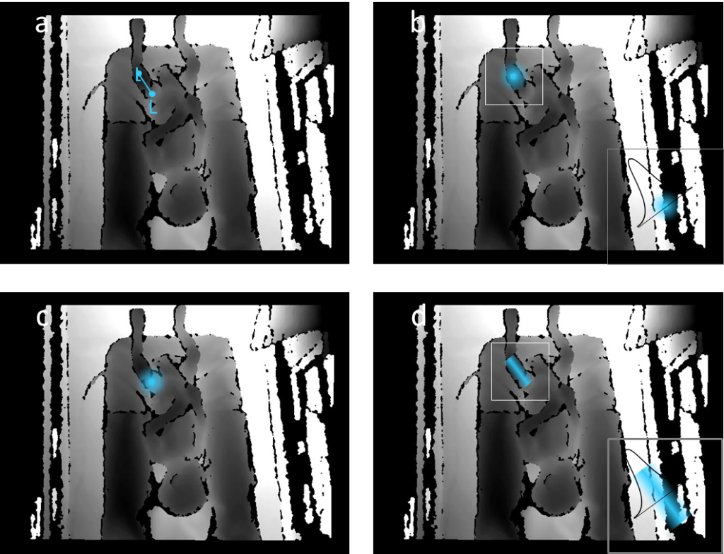
The regression CNN is fed by stacking the depth temporal clip and the corresponding affinity maps obtained from the detection network. Thus, the regression input is a 4D datum of dimension W x H x Wd x 21 (i.e., 1 depth channel +
12 joints + 8 connections). The regression network is trained with Wd x 20 ground-truth confidence maps of size W x H (Fig. 5). For every joint in each depth frame, we consider a region of interest consisting of all pixels that lie in the circle with radius r centered at the joint center. In this case, instead of binary masking the circle area as for the detection CNN, we consider a Gaussian distribution with standard deviation (σ) equal to 3*r and centered at the joint center. A similar approach is used to generate the ground-truth confidence maps for the joint connections. In this case, the ground-truth map is the rectangular region with thickness r and centrally aligned with the joint-connection line. Pixel values in the mask are 1-D Gaussian distributed (σ = 3*r) along the connection direction.
B. Spatio-temporal features for pose estimation
The proposed deep learning framework (Fig. 2) for spatiotemporal features computation for infants’ pose estimation consists of:
1) Detection network: Our architecture (Table II) is inspired by the classic encoder-decoder architecture of UNet [26], which is however implemented as a two-branch architecture for processing joints and joint connections separately. In fact, using a two-branch architecture has been shown to provide higher detection performance for 2D architecture [25], [8]. To incorporate the spatio-temporal information encoded in infants’ depth videos, we use 3D CNN kernels. The 3D convolution allows the kernel to move along the 3 input dimensions to process multiple frames at the same time, preserving and processing temporal information through the network.
Our detection network starts with an input layer and a common-branch convolutional layer (with stride = 1 and kernel size = 3x3x3 pixels), and is followed by 8 blocks. Each block TABLE II: Detection-network architecture. Starting from the input clip of Wd consecutive depth frames, the network generates Wd x 20 maps (for each frame of the clip: 12 and 8 affinity maps for joint and joint connections, respectively).
Name Kernel (Size / Stride) Channels W x1 3×3 / 1×1 W x64 Block 1 – Branch 1 2x2x2 / 2x2x1 Wdx64 3x3x3 / 1x1x1 Wdx64 Block 1 – Branch 2 2x2x2 / 2x2x1 Wdx64 3x3x3 / 1x1x1 Wdx64 Block 1 – Common branch 1x1x1 / 1x1x1 W Block 2 – Branch 1 2x2x2 / 2x2x1 3x3x2 / 1x1x1 Block 2 – Branch 2 2x2x2 / 2x2x1 3x3x3 / 1x1x1 Block 2 – Common branch 1x1x1 / 1x1x1 Block 3 – Branch 1 2x2x2 / 2x2x1 3x3x3 / 1x1x1 Block 3 – Branch 2 2x2x2 / 2x2x1 3x3x3 / 1x1x1 Block 3 – Common branch 1x1x1 / 1x1x1 Block 4 – Branch 1 2x2x2 / 2x2x2 3x3x3 / 1x1x1 Block 4 – Branch 2 2x2x2 / 2x2x1 3x3x3 / 1x1x1 Block 5 – Branch 1 2x2x2 / 2x2x1 Wdx256 3x3x3 / 1x1x1 Wdx256 Block 5 – Branch 2 2x2x2 / 2x2x1 Wdx256 3x3x3 / 1x1x1 Wdx256 Block 5 – Common branch 1x1x1 / 1x1x1 Wdx512 Block 6 – Branch 1 2x2x2 / 2x2x1 Wdx128 Block 4 – Common branch 1x1x1 / 1x1x1 Block 7 – Branch 1 2x2x2 / 2x2x1 Wdx64 3x3x3 / 1x1x1 Wdx64 Block 7 – Branch 2 2x2x2 / 2x2x1 Wdx64 3x3x3 / 1x1x1 Wdx64 Block 7 – Common branch 1x1x1 / 1x1x1 Wdx128 Block 8 – Branch 1 2x2x2 / 2x2x1 Wdx32 3x3x3 / 1x1x1 Wdx32 Block 8 – Branch 2 2x2x2 / 2x2x1 Wdx32 3x3x3 / 1x1x1 Wdx32 Block 8 – Common branch 1x1x1 / 1x1x1 Wdx64 1x1x1/1x1x1 Wdx20 3x3x3 / 1x1x1 W Block 6 – Branch 2 2x2x2 / 2x2x1 3x3x3 / 1x1x1 Block 6 – Common branch 1x1x1 / 1x1x1 TABLE III: Regression-network architecture. The network is fed with Wd consecutive depth frames (each with 1 channel) stacked with the corresponding (20) affinity maps from the detection network, and produces Wdx20 confidence maps (12 for joints and 8 for connections, for each of the Wd input frames). Name Kernel (Size / Stride) Channels Input — Wd x21 Layer 1 3x3x3 / 1x1x1 Wdx64 Layer 2 3x3x3 / 1x1x1 Wdx128 Layer 3 3x3x3 / 1x1x1 Wdx256 Layer 4 3x3x3 / 1x1x1 Wdx256 Layer 5 1x1x1 / 1x1x1 Wdx256 Output 1x1x1 / 1x1x1 Wdx20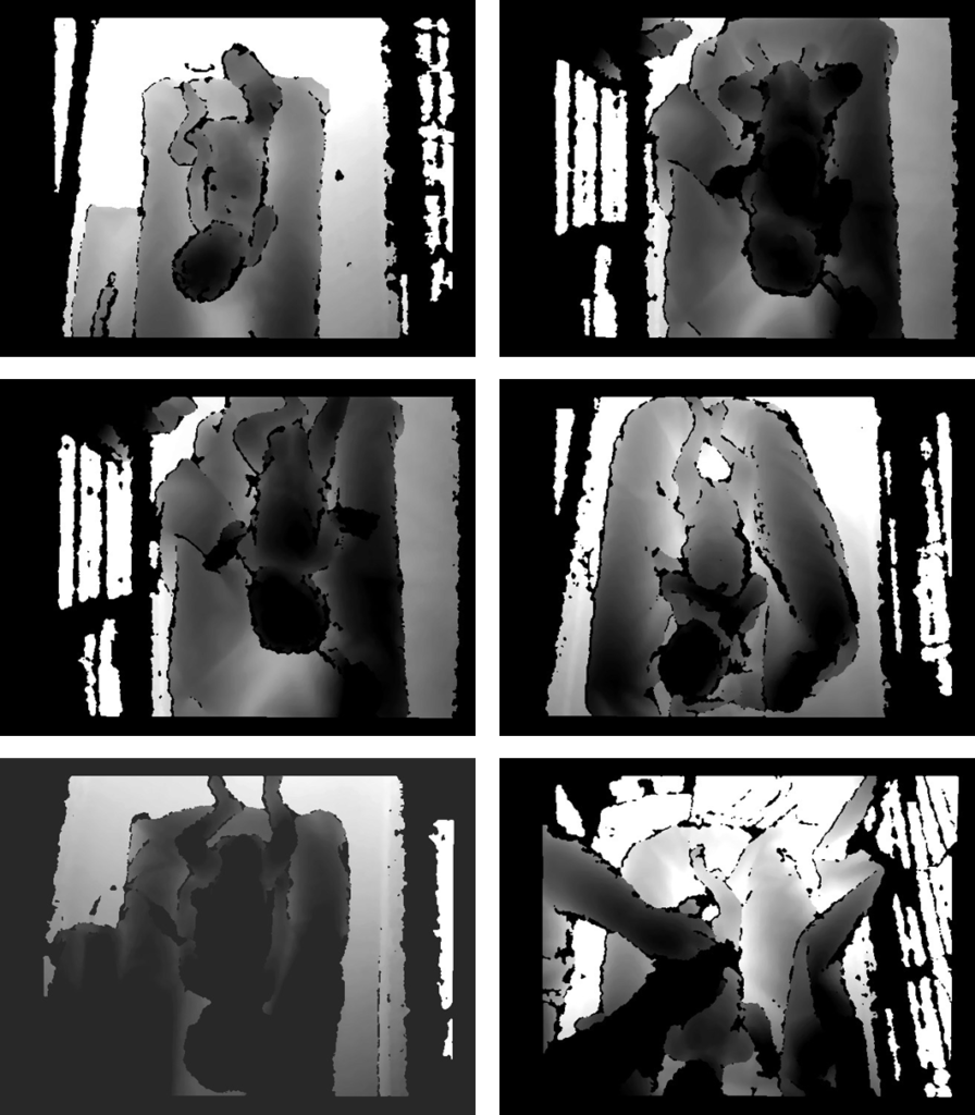
Is first divided in two branches (for joints and connections). In each branch, two convolutions are performed: the former with kernel size = 2x2x2 and stride 2x2x1, while the latter with kernel size = 3x3x3 and stride 1x1x1. It is worth noting that we set the kernel stride equal to 1 in the temporal dimension as to avoid deteriorating meaningful temporal information. The outputs of the two branches in a block are then concatenated in a single output, prior entering the next block. In each block of the encoder path, the number of channels is doubled. Batch normalization and activation with the rectified linear unit (ReLu) are performed after each convolution.
The architecture of the decoder path is symmetric to the encoder one and ends with an output layer with Wdx20 channels (12 for joints and 8 for connections) activated with the sigmoid function.
Our detection CNN is trained using the adaptive moment estimation (Adam) as optimizer and the per-pixel binary crossentropy (LCE), adapted for multiple 3D map training, as loss function:

where pt,k(x) and p˜t,k(x) are the ground-truth affinity maps and the corresponding output at pixel location x in the depthframe domain (Ω) of channel k for temporal frame t, J=12 and C=8 are the number of joints and joint connections, respectively.
2) Regression network: The necessity of using a regression network for the addressed task comes from considerations of previous work [27], which showed that directly regressing joint position from an input frame is highly non linear. Our regression network, instead, produces Wdx20 stacked confidence maps (12 for joints and 8 for connections). Each map has the same size of the input depth clip (i.e., WxH).
Also in this case, 3D convolution is performed to exploit spatio-temporal features. The newtork consists of five layers of 3x3x3 convolutions (Table III). Kernel stride is always set to 1, to preserve the spatio-temporal resolution. In the first 3 layers, the number of activations is doubled, ranging from 64 to 256. The number of activations is then kept constant for the last two layers. Batch normalization and ReLu-activation are performed after each 3D convolution.
Our regression network is trained with the stochastic gradient descent as optimizer using the mean squared error (LMSE), adapted for multiple 3D map training, as loss function:

where ht,k(x) and h˜t,k(x) are the ground truth and the predicted value at pixel location x of the kth channel for temporal frame t, respectively.
3) Joint linking: The last step of our limb pose-estimation task is to link subsequent joints for each of the infants’ limb, which is done on depth images, individually. First, we identify joint candidates from the output joint-confidence maps using non-maximum suppression, which is an algorithm commonly used in computer vision when redundant candidates are present [28]. Once joint candidates are identified, they are linked exploiting the joint-connection confidence maps. In particular, we use a bipartite matching approach, which consists of: (i) computing the integral value along the line connected two candidates on the joint-connection confidence map and (ii) choosing the two winning candidates as those guaranteeing the highest integral value.
III. EVALUATION
A. Dataset
Our babyPose dataset consisted of 16 depth videos of 16 preterm infants that were acquired in the NICU of the G. Salesi Hospital in Ancona, Italy. The infants were identified by clinicians in the NICU among those who were spontaneously breathing. Written informed consent was obtained from the infant’s legal guardian.
Video-acquisition setup, which is shown in Fig. 1, was designed to not hinder healthcare operators in their work activities. The 16 video recordings (length = 180s) were acquired for every infant using the Astra Mini S – Orbbec R , with a frame rate of 30 frames per second and image size of 640×480 pixels. No frame selection was performed (i.e., all frames were used for the analysis).
| TABLE IV: Joint-detection performance in terms of median Dice similarity coefficient (DSC) and recall (Rec). Inter-quartile range is reported in brackets. The metrics are reported separately for each joint. For joint acronyms, refer to the joint-pose model in Fig. 3. Right arm Left arm Right leg Left leg RWRERSLSLELWRARKRHLHLKLA DSC 2D0.84 (0.11)0.87 (0.10)0.86 (0.09)0.87 (0.09)0.85 (0.08)0.86 (0.09)0.86 (0.10)0.87 (0.07)0.84 (0.08)0.85 (0.09)0.86 (0.07)0.87 (0.07)3D0.93 (0.06)0.94 (0.06)0.94 (0.07)0.94 (0.08)0.94 (0.06)0.94 (0.06)0.93 (0.06)0.94 (0.05)0.93 (0.06)0.93 (0.06)0.94 (0.05)0.93 (0.06) Rec 2D0.73 (0.15)0.77 (0.15)0.76 (0.11)0.78 (0.13)0.73 (0.11)0.76 (0.14)0.77 (0.15)0.78 (0.11)0.73 (0.11)0.74 (0.12)0.76 (0.12)0.78 (0.10)3D0.89 (0.11)0.90 (0.10)0.91 (0.11)0.91 (0.12)0.90 (0.09)0.90 (0.09)0.89 (0.09)0.90 (0.09)0.88 (0.09)0.89 (0.09)0.92 (0.07)0.89 (0.11)TABLE V: Joint-connection detection performance in terms of median Dice similarity coefficient (DSC) and recall (Rec). Inter-quartile range is reported in brackets. The metrics are reported separately for each joint connection. For joint acronyms, refer to the joint-pose model in Fig. 3. Right armLeft armRight legLeft leg RW-RERE-RSLS-LELE-LWRA-RKRK-RHLH-LKLK-LA DSC 2D0.89 (0.08)0.90 (0.08)0.89 (0.07)0.88 (0.08)0.90 (0.06)0.88 (0.08)0.90 (0.07)0.91 (0.06)3D0.93 (0.06)0.93 (0.08)0.94 (0.08)0.94 (0.06)0.93 (0.05)0.93 (0.06)0.94 (0.06)0.94 (0.06) Rec 2D0.81 (0.12)0.84 (0.13)0.81 (0.12)0.81 (0.12)0.85 (0.09)0.80 (0.12)0.85 (0.12)0.85 (0.09)3D0.90 (0.10)0.89 (0.15)0.92 (0.13)0.90 (0.10)0.90 (0.08)0.88 (0.09)0.91 (0.09)0.902 (0.10) |
Joint annotation was performed using a custom-built annotation tool, publicly available online[1]. For each video, the annotation was manually obtained every 5 frames, until 1000 frames per infant were annotated. In accordance with our clinical partners, performing manual annotation every 5 frames may be considered a good compromise considering the average preterm infants’ movement rate [29]. Then, these 1000 frames were split into training and testing data: 750 frames were used for training purpose and the remaining ones (250 frames) to test the network; resulting in a training set of 12000 samples (16 infants x 750 frames) and a testing set of 4000 samples (16 infants x 250 frames). From the 12000 training samples, we kept 200 frames for each infant as validation set, for a total of 3200 frames.
Figure 6 shows some of the challenges in the dataset, such as varying infant-camera distance (due to the motility of the acquisition setup), different number of visible joints (due to partial or total limb occlusion) and presence of homogeneous areas with similar or at least continuous intensity values, due to the use of the depth video.
B. Training settings
All frames were resized to 128×96 pixels in order to smooth noise and reduce both training time and memory requirements. Mean intensity was removed from each frame. To build the ground-truth masks, we selected rd equal to 6 pixels, as to completely overlay the joints. The Ws was set to 2 for training and 0 for testing, while Wd was set to 3. This way, a temporal clip was 0.5s long.
For training the detection and regression network, we set an initial learning rate of 0.01 with a learning decay of 10% every 10 epochs, and a momentum of 0.98. We used a batch size of
8 and set a number of epochs equal to 100. We selected the best model as the one that maximized the detection accuracy and minimized the mean absolute error on the validation set, for the detection and regression network, respectively. All our analyses were performed using Keras[2]on a Nvidia GeForce GTX 1050 Ti/PCIe/SSE2.
C. Comparison with spatial features and ablation study
We decided to compare the performance of the proposed spatio-temporal features with that of spatial features alone. We chose the closest work with respect to ours [20], which uses the same architectures presented in Table IV and Table V, but with 2D spatial convolution.
For the ablation study, inspired by [30], we compared the performance of the proposed framework with the detectiononly and regression-only architectures. Both were implemented in a spatio-temporal fashion (i.e., with 3D convolution). For the detection-only model, the affinity maps were used to directly estimate limb pose with the bipartite-matching strategy described in Sec. II-B3. The regression-only model was fed with the depth clips and trained with the confidencemap ground truth. The output was then used to estimate joint pose with bipartite matching.
D. Performance metrics
To measure the performance of the detection network, as suggested in [8], we computed the Dice similarity coefficient (DSC) and recall (Rec), which are defined as:
 (3)
(3)
 (4)
(4)
| TABLE VI: Limb-pose estimation performance in terms of median root mean square distance (RMSD), with interquartile range in brackets, computed with respect to the ground-truth pose. The RMSD is reported for each limb, separately. Results are reported for the 2D and 3D framework, as well as for the 3D detection-only and 3D regression-only architectures. Right armLeft armRight legLeft leg RMSD 2D11.73 (3.58)10.54 (4.97)11.03 (5.78)11.50 (4.21)Detection-only network15.09 (3.80)15.60 (3.87)15.09 (3.41)14.91 (3.49)Regression-only network12.39 (2.18)11.73 (3.25)11.95 (4.60)12.17 (2.47)3D9.76 (4.60)9.29 (5.89)8.90 (5.64)9.20 (3.99) |
(a) Joint Rec
(b) Joint-connetction Rec
where TP and FP are the true joint and background pixels detected as joints, respectively, while FN refers to joint pixels that are detected as background. The same applied to joint connections.
To evaluate the overall pose estimation, we computed the root mean square distance (RMSD) [pixels] for each infants’ limb. For both the detection and regression network, we measured the testing time.
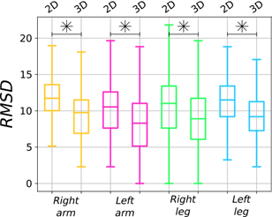
Two-sided t-test with significance level (α) = 0.05 was used to evaluate if significative differences were present between the 2D and 3D framework in estimating limb pose.
IV. RESULTS
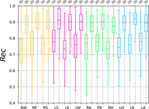
The descriptive statistics of Rec and DSC for the detection CNN are reported in Table IV. Figure 7a shows the Rec boxplots for joints. Results are also shown for the corresponding 2D implementation. The highest median DSC (0.94, interquartile range (IQR) = 0.05) among all joints was obtained with the 3D CNN. The same was observed for the Rec, with a median value among all joints of 0.90, and IQR of 0.09. Note that, in the case yielding the least accurate result, which corresponds to the RH joint, the Rec still achieved 0.88, whereas for the 2D detection network the lowest Rec was 0.73. The same behaviour (Table V and Fig. 7b) was observed when considering the joint-connection detection performance, with median DSC = 0.93 (IQR = 0.06) and median Rec = 0.90 (IQR = 0.11) among all connections.
The performance comparison in terms of RMSD of the different models presented in Sec. III-C is summarized in Table VI. The highest performance (i.e., the lowest RMSD) was achieved by the 3D framework, with a median value of 9.06 pixels (IQR = 5.12) among the four limbs. The best performance was achieved for the right leg (median = 8.90 pixels, IQR = 5.64 pixels). The overall computational time for our 3D framework was 0.06s per image on average. The 2D framework always showed lower performance, with the best and worst RMSD equal to 10.54 (left arm) and 11.73 (right arm) pixels, respectively (median among the four limbs = 11.27 with IQR = 4.59). The overall statistics are shown in Fig. 8. The results all differed significantly (p-value < α) from those obtained with the 3D framework. The detection-only and regression-only networks showed the lowest performance, with a median RMSD equal to 15.09 pixels and 12.06 pixels, respectively.
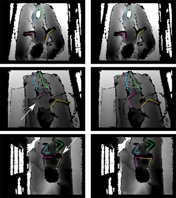
In Fig. 9, qualitative results for infants’ pose estimation are shown both for the 2D framework (on the left side) and the 3D one (on the right side). The white arrows highlight errors in pose estimation made by the 2D framework. Results of the 3D framework for challenging cases are shown in Fig. 10. The first row shows samples in which one joint was not detected due to auto-occlusion. Joints were also not detected when external occlusion occurred (second row), due to the interaction of the healthcare-operator with the infant or to the presence of plaster. The proposed framework was not able to produce joint estimation also when image noise and intensity inhomogeneities (e.g., due to rapid infants movement) were present (third row). At the same time, however, other joints in the image were correctly estimated thanks to the joint-map parallel processing.
V. DISCUSSION
Monitoring preterm infants’ limb is crucial for assessing infant’s health status and early detecting cognitive/motor disorders. However, when surveying the clinical literature, we realized that there is a lack of documented quantitative parameters on the topic. This is mainly due to the drawbacks of current monitoring techniques, which rely on qualitative visual judgment of clinicians at the crib side in NICUs. A possible, straightforward, solution may be to exploit contact sensors (such as accelerometers). Nonetheless, in NICUs, using additional hardware may contribute significantly to infants’ stress, discomfort and pain and, from the healthcare operators’ point of view, may hinder the actual clinical practice. To overcome all these issues, researchers seek for new reliable and unobtrusive monitoring alternatives, which are mostly based on video analysis. With this paper, we proposed a novel framework for non-invasive monitoring of preterm infants’ limbs through providing an innovative approach for limb-pose estimation from spatio-temporal features extracted from depth videos. We decided to exploit depth videos (over approaches based on RGB videos) to accomplish considerations relevant to privacy protection. The deep learning framework was validated on a dataset of 16 preterm infants, whose video recordings, acquired in the actual clinical practice, presented several challenges such as: presence of homogeneous areas with similar or at least continuous intensity, self- or external occlusions and different pose of the camera with respect to the infants.
The proposed 3D detection network achieved encouraging results as shown in Fig. 7 and reported in Table IV, with a median DSC of 0.94 and 0.93 for joint and joint-connection, respectively, overcoming our previous approach based on spatial features only [20]. The network performed comparably when detecting all joints and joint-connection as shown by the IQRs in Table IV, reflecting the CNN ability of processing in parallel the different joint and joint-connection affinity maps.
The 3D framework achieved improved performance (Table VI) in estimating infants’ pose for all limbs (median RMSD = 9.06 pixels) when compared with our previous 2D approach (median RMSD = 11.27 pixels). These results suggest that exploiting temporal information improved network generalization ability even in presence of intensity homogeneity and noisy background, typical of depth images. These considerations are visible in Fig. 9, where the 2D framework failed in detecting joints that lay in portions of the image with homogeneous intensity.
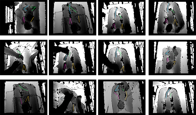
First row: one joint was not detected due to auto-occlusion (from left to right: right shoulder, right shoulder, right hip, right hip). Second row: one or more joints were not detected due to external occlusion (from left to right: joint of the left limbs, right ankle, left arm – due to healthcare operator hand presence, and right knee and ankle – due to plaster). Last row: image noise and intensity inhomogeneities prevented joint detection.
Predictions of the pose estimation were computed also for the detection- (median RMSD = 15.09 pixels) and the regression-only networks (median RMSD = 12.06 pixels). Despite the complexity of regressing joint and jointconnection confidence maps from depth image clips only, the regression-only network achieved better results when compared to the detection-only network. The lower performance of the detection-only network may be due to the complexity in localizing joint candidates from ground-truth binary masks, where all pixels have the same weight (Fig. 4). It is worth noting that spatio-temporal features were tested for a detectiononly task in [8] (even though for surgical instrument joints in laparoscopic video). Here, however, we moved forward to test joint estimation by combining the detection network with bipartite matching, and comparing the achieved results with the full 3D detection+regression framework. Despite the integration of the temporal information, both the detectiononly and regression-only network achieved lower outcomes with respect to the full 2D framework. Hence, the regressiononly model was barely capable of predicting the location of joints without any guidance. Regression is empirically too localized (i.e., it supports small spatial context) and the process of regressing from original input image to joint location directly is challenging. By combining detection and regression, the detection module acted as structural guidance for the regression module by providing spatial contextual information between joints, and facilitating the joints localization.
A straightforward limitation of this work may be seen in the estimation of occluded joints (both in case of auto and external occlusion), as shown in Fig. 10 (first and second rows). At the same time, our two-branch architecture with multiple maps allowed to detect the other (not-occluded) joints in the image. This issue could be attenuated with recent strategies proposed in the literature for long-term tracking [31] and confidence estimation [32]. Modeling infant’ limbs through anthropometric measures (such as limb length – already acquired in the actual clinical practice) could also help in attenuating the occlusion issue. This would probably also make our 3D framework able to tackle noisy image portions, which may be present due to sudden movement of infants or healthcare operators (Fig. 10, last row). We also recognize that a limitation of the proposed work could be seen is the relatively limited number of testing frames (4000), which is due to the lack of available annotated dataset online. To attenuate this issue, we released the data we collected for further use in the community. Natural extensions of the proposed work deal with the inclusion of the limbpose estimation within other computed-assisted algorithms for diagnostic support, e.g. to classify abnormal limb movements. The proposed acquisition setup could be also integrated with recent video-based monitoring systems for respiratory rate analysis [33].
VI. CONCLUSION
In this paper, we proposed a framework for preterm infants’ limb-pose estimation from depth images based on spatiotemporal features. Our results, achieved by testing a new contribution dataset (which is also the first in the field), suggest that spatio-temporal features can be successfully exploited to increase pose-estimation performance with respect to 2D models based on single-frame (spatial only) information.
In conclusion, our solution moves us towards a better framework for preterm infants’ movement understanding and can lead to applications in computer-assisted diagnosis. Moreover, by making our dataset fully available, we believe we will stimulate researches in the field, encouraging and promoting the clinical translation of preterm infants’ monitoring systems for timely diagnosis and prompt treatment.
Compliance with ethical standards Disclosures
The authors have no conflict of interest to disclose.
Ethical standards
The procedures followed were in accordance with the ethical standards of the responsible committee on human experimentation (institutional and national) and with the Helsinki Declaration of 1975, as revised in 2000. This article followed the Ethics Guidelines for Trustworthy Artificial Intelligence, recently published by the European Commission[3].
REFERENCES
[1] A. Polito, S. Piga, P. E. Cogo, C. Corchia, V. Carnielli, M. Da Fre,` D. Di Lallo, I. Favia, L. Gagliardi, F. Macagno et al., “Increased morbidity and mortality in very preterm/VLBW infants with congenital heart disease,” Intensive Care Medicine, vol. 39, no. 6, pp. 1104–1112, 2013.
[2] C. Einspieler, H. F. Prechtl, F. Ferrari, G. Cioni, and A. F. Bos, “The qualitative assessment of general movements in preterm, term and young infants—review of the methodology,” Early Human Development, vol. 50, no. 1, pp. 47–60, 1997.
[3] F. Ferrari, C. Einspieler, H. Prechtl, A. Bos, and G. Cioni, Prechtl’s method on the qualitative assessment of general movements in preterm, term and young infants. Mac Keith Press, 2004.
[4] T. Moore, S. Johnson, S. Haider, E. Hennessy, and N. Marlow, “Relationship between test scores using the second and third editions of the Bayley Scales in extremely preterm children,” The Journal of Pediatrics, vol. 160, no. 4, pp. 553–558, 2012.
[5] I. Bernhardt, M. Marbacher, R. Hilfiker, and L. Radlinger, “Interand intra-observer agreement of Prechtl’s method on the qualitative assessment of general movements in preterm, term and young infants,” Early Human Development, vol. 87, no. 9, pp. 633–639, 2011.
[6] D. G. Sweet, V. Carnielli, G. Greisen, M. Hallman, E. Ozek, R. Plavka, O. D. Saugstad, U. Simeoni, C. P. Speer, M. Vento et al., “European consensus guidelines on the management of respiratory distress syndrome2016 update,” Neonatology, vol. 111, no. 2, pp. 107–125, 2017.
[7] ——, “European consensus guidelines on the management of neonatal respiratory distress syndrome in preterm infants-2013 update,” Neonatology, vol. 103, no. 4, pp. 353–368, 2013.
[8] E. Colleoni, S. Moccia, X. Du, E. De Momi, and D. Stoyanov, “Deep learning based robotic tool detection and articulation estimation with spatio-temporal layers,” IEEE Robotics and Automation Letters, vol. 4, no. 3, pp. 2714–2721, 2019.
[9] D. Tran, H. Wang, L. Torresani, J. Ray, Y. LeCun, and M. Paluri, “A closer look at spatiotemporal convolutions for action recognition,” in IEEE Conference on Computer Vision and Pattern Recognition, 2018, pp. 6450–6459.
[10] A. Karpathy, G. Toderici, S. Shetty, T. Leung, R. Sukthankar, and L. Fei-Fei, “Large-scale video classification with convolutional neural networks,” in IEEE Conference on Computer Vision and Pattern Recognition, 2014, pp. 1725–1732.
[11] A. Hernandez-Vela, N. Zlateva, A. Marinov, M. Reyes, P. Radeva,´ D. Dimov, and S. Escalera, “Graph cuts optimization for multi-limb human segmentation in depth maps,” in IEEE Conference on Computer Vision and Pattern Recognition. IEEE, 2012, pp. 726–732.
[12] I. Trujillo-Priego, C. Lane, D. Vanderbilt, W. Deng, G. Loeb, J. Shida, and B. Smith, “Development of a wearable sensor algorithm to detect the quantity and kinematic characteristics of infant arm movement bouts produced across a full day in the natural environment,” Technologies, vol. 5, no. 3, p. 39, 2017.
[13] B. Smith, I. Trujillo-Priego, C. Lane, J. Finley, and F. Horak, “Daily quantity of infant leg movement: wearable sensor algorithm and relationship to walking onset,” Sensors, vol. 15, no. 8, pp. 19006–19020, 2015.
[14] C. Jiang, C. J. Lane, E. Perkins, D. Schiesel, and B. A. Smith, “Determining if wearable sensors affect infant leg movement frequency,” Developmental Neurorehabilitation, vol. 21, no. 2, pp. 133–136, 2018.
[15] A. Cenci, D. Liciotti, E. Frontoni, A. Mancini, and P. Zingaretti, “Non-contact monitoring of preterm infants using RGB-D camera,” in International Design Engineering Technical Conferences and Computers and Information in Engineering Conference. American Society of Mechanical Engineers, 2015, pp. V009T07A003–V009T07A003.
[16] S. Orlandi, K. Raghuram, C. R. Smith, D. Mansueto, P. Church, V. Shah, M. Luther, and T. Chau, “Detection of atypical and typical infant movements using computer-based video analysis,” in Annual International Conference of the IEEE Engineering in Medicine and Biology Society. IEEE, 2018, pp. 3598–3601.
[17] D. Freymond, Y. Schutz, J. Decombaz, J.-L. Micheli, and E. Jequier,´ “Energy balance, physical activity, and thermogenic effect of feeding in premature infants,” Pediatric Research, vol. 20, no. 7, p. 638, 1986.
[18] M. Khan, M. Schneider, M. Farid, and M. Grzegorzek, “Detection of infantile movement disorders in video data using deformable part-based model,” Sensors, vol. 18, no. 10, p. 3202, 2018.
[19] Y. LeCun, Y. Bengio, and G. Hinton, “Deep learning,” Nature, vol. 521, no. 7553, p. 436, 2015.
[20] S. Moccia, L. Migliorelli, R. Pietrini, and E. Frontoni, “Preterm infants’ limb-pose estimation from depth images using convolutional neural networks,” in IEEE International Conference on Computational Intelligence in Bioinformatics and Computational Biology. IEEE, in press.
[21] H. Rahmati, R. Dragon, O. M. Aamo, L. Adde, Ø. Stavdahl, and L. Van Gool, “Weakly supervised motion segmentation with particle matching,” Computer Vision and Image Understanding, vol. 140, pp. 30–42, 2015.
[22] R. Hou, C. Chen, and M. Shah, “An end-to-end 3D convolutional neural network for action detection and segmentation in videos,” arXiv preprint arXiv:1712.01111, 2017.
[23] C. B. Heriza, “Comparison of leg movements in preterm infants at term with healthy full-term infants,” Physical Therapy, vol. 68, no. 11, pp. 1687–1693, 1988.
[24] T. H. Kakebeeke, K. von Siebenthal, and R. H. Largo, “Differences in movement quality at term among preterm and term infants,” Neonatology, vol. 71, no. 6, pp. 367–378, 1997.
[25] Z. Cao, T. Simon, S.-E. Wei, and Y. Sheikh, “Realtime multi-person 2D pose estimation using part affinity fields,” in Conference on Computer Vision and Pattern Recognition, 2017, pp. 7291–7299.
[26] O. Ronneberger, P. Fischer, and T. Brox, “U-net: Convolutional networks for biomedical image segmentation,” in International Conference on Medical Image Computing and Computer-Assisted Intervention. Springer, 2015, pp. 234–241.
[27] A. Bulat and G. Tzimiropoulos, “Human pose estimation via convolutional part heatmap regression,” in European Conference on Computer Vision. Springer, 2016, pp. 717–732.
[28] J. Hosang, R. Benenson, and B. Schiele, “Learning non-maximum suppression,” in IEEE Conference on Computer Vision and Pattern Recognition, 2017, pp. 4507–4515.
[29] B. Fallang, O. D. Saugstad, J. Grøgaard, and M. Hadders-Algra, “Kinematic quality of reaching movements in preterm infants,” Pediatric Research, vol. 53, no. 5, p. 836, 2003.
[30] X. Du, T. Kurmann, P.-L. Chang, M. Allan, S. Ourselin, R. Sznitman, J. D. Kelly, and D. Stoyanov, “Articulated multi-instrument 2-D pose estimation using fully convolutional networks,” IEEE Transactions on Medical Imaging, vol. 37, no. 5, pp. 1276–1287, 2018.
[31] V. Penza, X. Du, D. Stoyanov, A. Forgione, L. S. Mattos, and E. De Momi, “Long term safety area tracking (LT-SAT) with online failure detection and recovery for robotic minimally invasive surgery,” Medical Image Analysis, vol. 45, pp. 13–23, 2018.
[32] S. Moccia, S. J. Wirkert, H. Kenngott, A. S. Vemuri, M. Apitz, B. Mayer, E. De Momi, L. S. Mattos, and L. Maier-Hein, “Uncertainty-aware organ classification for surgical data science applications in laparoscopy,” IEEE Transactions on Biomedical Engineering, vol. 65, no. 11, pp. 2649– 2659, 2018.
[33] C. B. Pereira, X. Yu, T. Goos, I. Reiss, T. Orlikowsky, K. Heimann, B. Venema, V. Blazek, S. Leonhardt, and D. Teichmann, “Noncontact monitoring of respiratory rate in newborn infants using thermal imaging,” IEEE Transactions on Biomedical Engineering, vol. 66, no. 4, pp.
1105–1114, 2018.
[1] https://github.com/roccopietrini/pyPointAnnotator
[2] https://keras.io/
[3] https://ec.europa.eu/futurium/en/ai-alliance-consultation